A fun video of highly composite numbers:
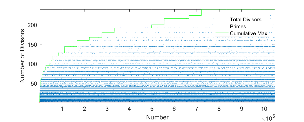
And a plot from MATLAB displaying increasing numbers and their number of divisors up to 2^20.
Development, Research, Other Stuff
A fun video of highly composite numbers:
And a plot from MATLAB displaying increasing numbers and their number of divisors up to 2^20.

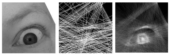 A recent post I saw here demonstrated an artists technique of plotting lines across a page so that a series of lines pass through the entire page and together create a recognizable image. This post demonstrates a recreation of the technique using software.
Results are above (original, basic render, buildup render), and the references art image:
I initially wanted to perform an exhaustive search of possible lines in the image, or find existing lines using something like a Hough Transform or curvelets. However, the exhaustive search of possible lines at each iteration was slow and complicated, so I ended up just test a couple hundred lines from a random edge to random edge and greedily minimize the remaining energy in the image.
The first iteration simply made a line across the image with magnitude one. This results of a very rough image:
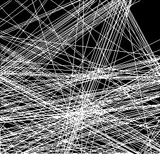
The next iteration allows the lines to build up, so lines can become darker and dark with each stroke. This results in a much nicer image while still requiring that each line fall across the entire image from edge to edge.
An interesting extension would be to choose a few colors and process a blue channel, as with the original author, rather than just processing grayscale.

Click to Download Presentation
L1-Magic is old interior-point library developed by Justin Romberg around 2005. It solves seven problems related to compressive sensing and the convex relaxation of L0 problems:
In the attached presentation given to the Georgia Tech CSIP Compressed Sensing Group and the So-Called “Children of the Norm”, I show how modifications to a handful of lines of code in L1-Magic can result in
To do this, I use the following limitations
The improvements are made to Basis Pursuit, L1 with Quadratic Constraints, and TV1 with various degrees of success:
One substantial contribution is that the l1qc (P2) code displayed substantial stability issues. For low rank problems, we completely fix this issue and show ~100x speedup on certain problems. Results are dependent on the shape of A (low rank gives us better results) and incorporating these results may require switching methods between the current implementation and these proposed changes as m approaches n.

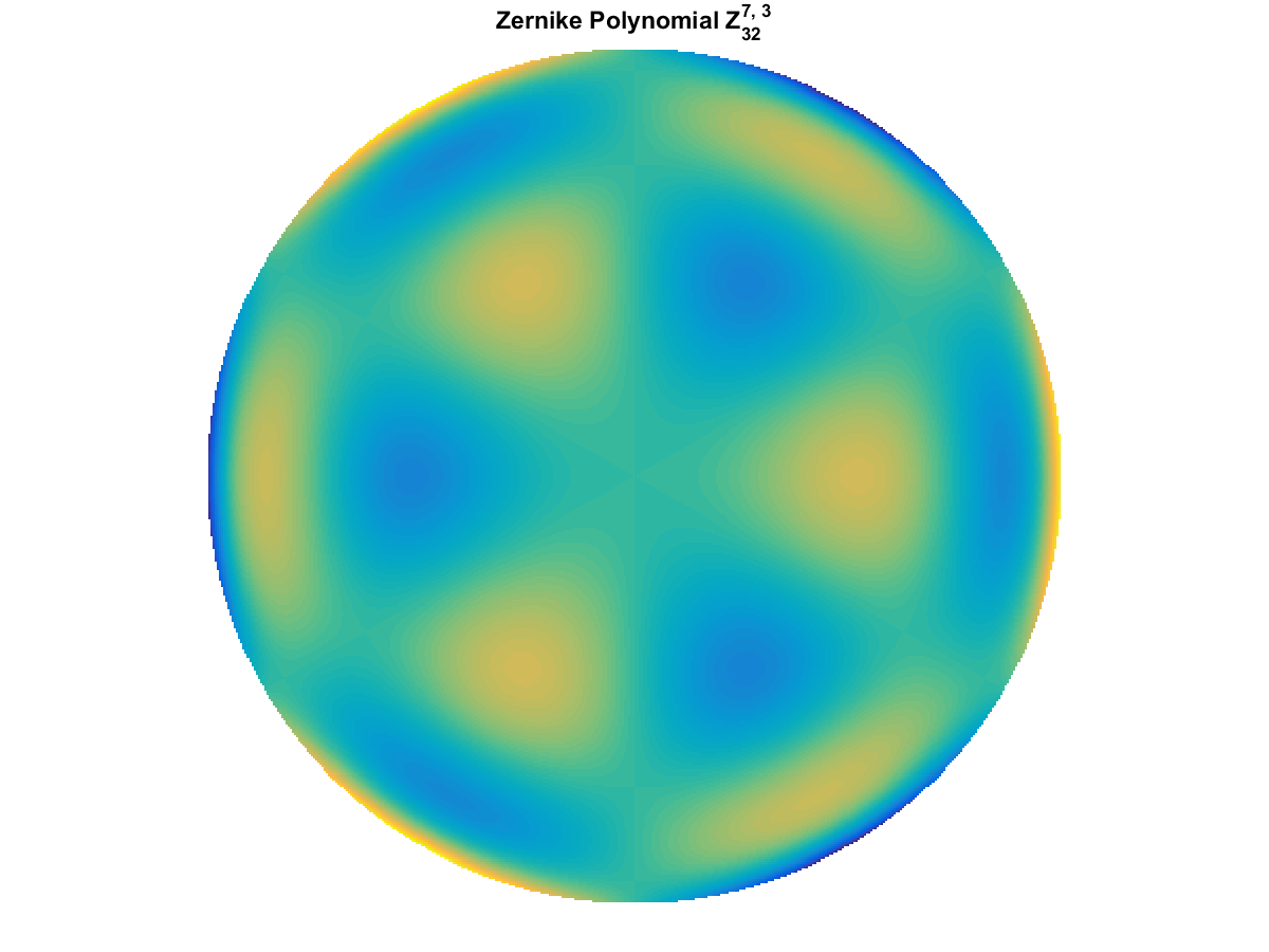
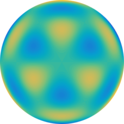
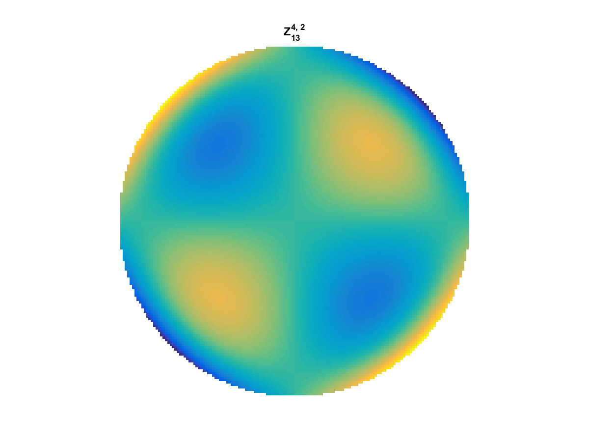
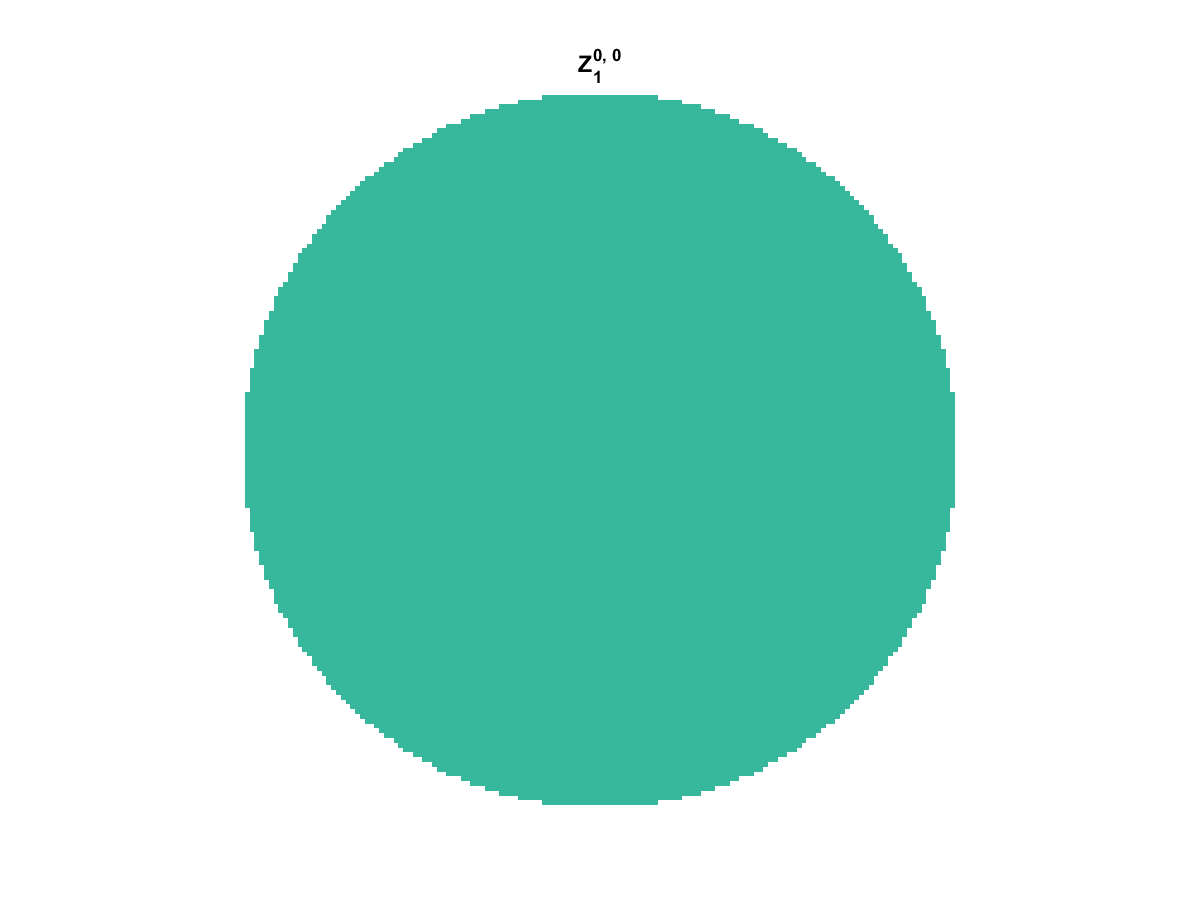
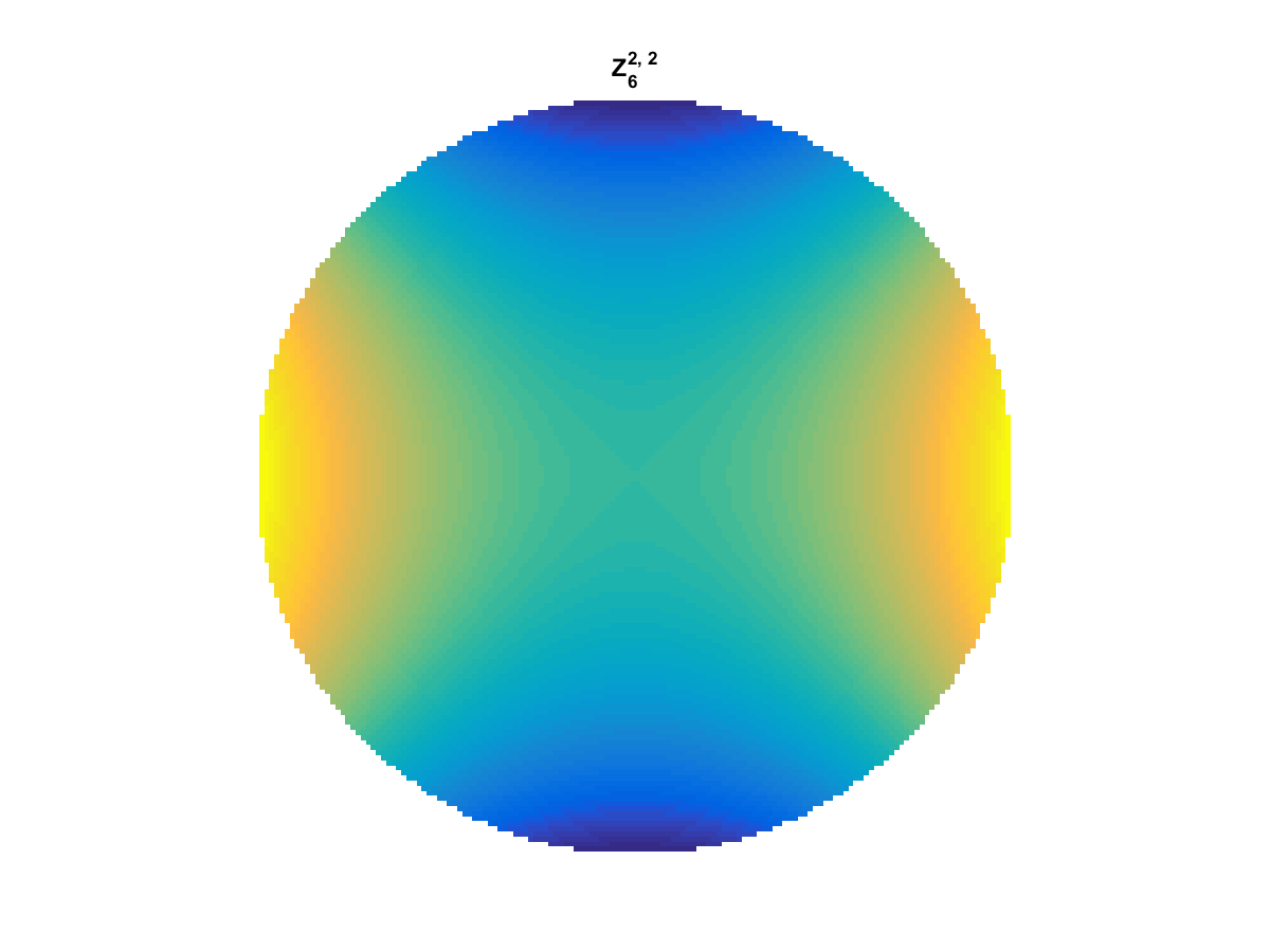
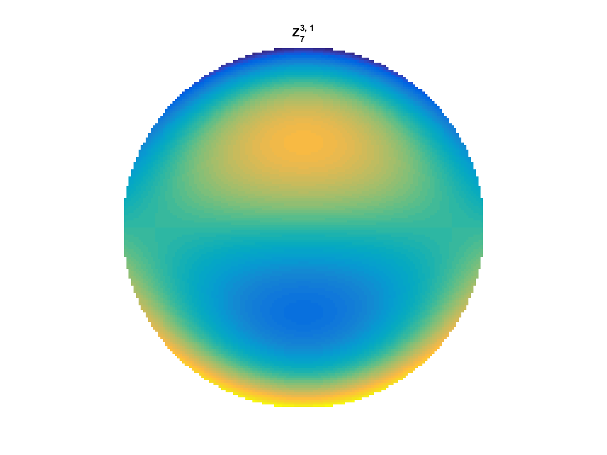
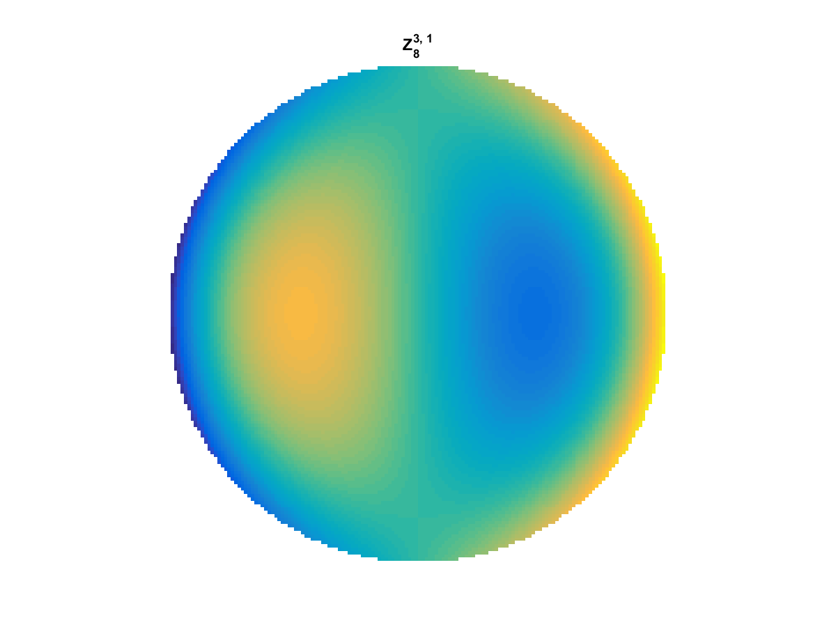
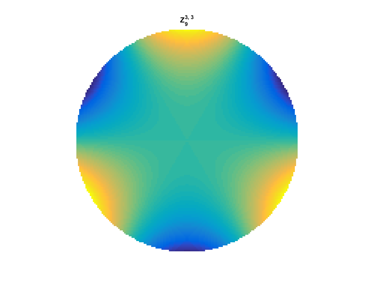
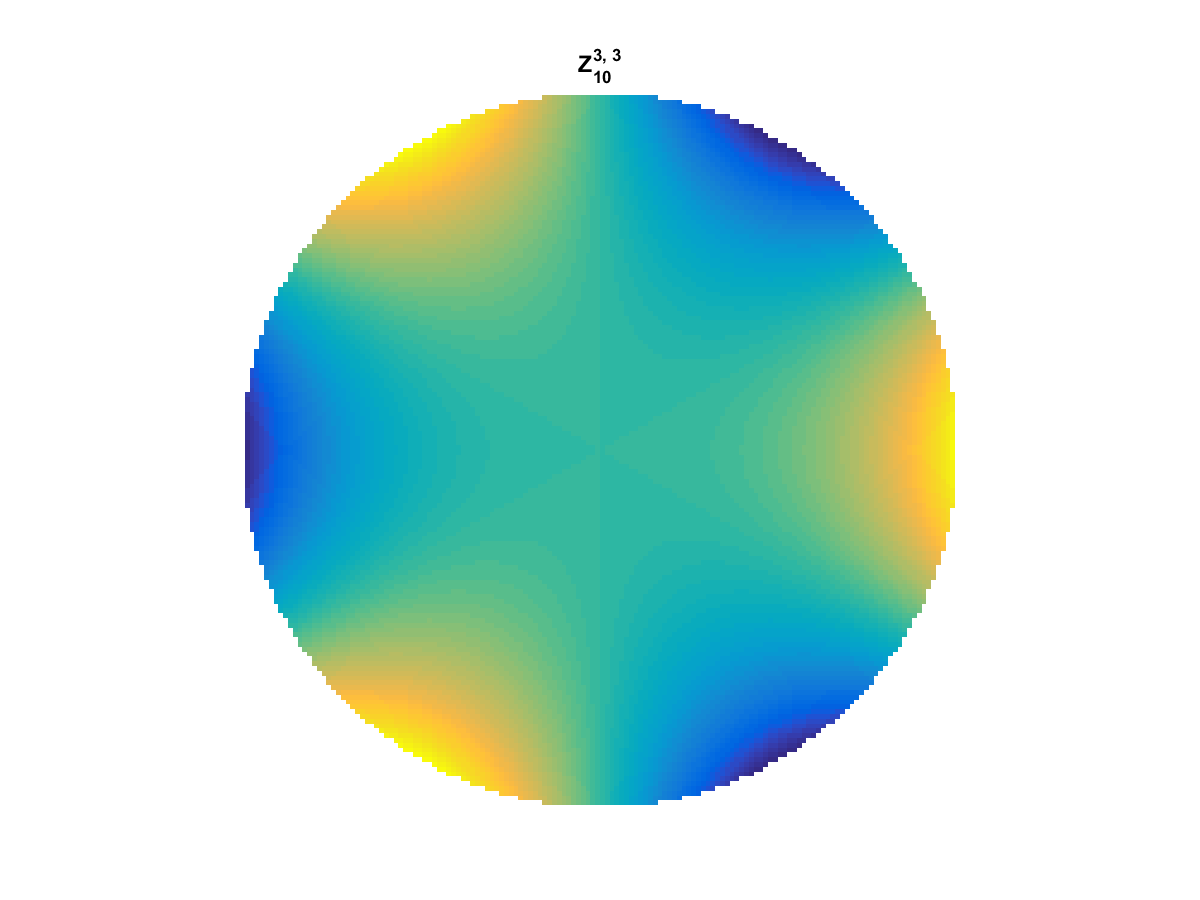
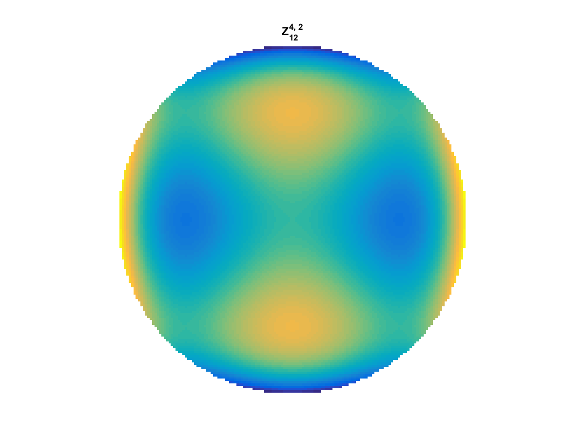
A quick implementation of of Zernike polynomials for modeling wavefront aberrations to to optical turbulence. Equations pulled from Michael Roggemann’s Imaging Through Turbulence.
Zernike polynomials are often used to model wavefront aberrations for various optics problems. The equations are expressed in polar coordinates, so to calculate the image we first convert a grid into polar coordinates using the relation
\(y = r\times sin(\theta) \)
\(r = \sqrt{x^2 + y^2} \)
\(\theta = tan^{-1}\frac{y}{x}\)
And then calculate the Zernike Polynomials as
\(Z_{i,even}(r,\theta) = \sqrt{n+1}R^m_n(r)cos(m\theta) \)
\(Z_{i,odd}(r,\theta) = \sqrt{n+1}R^m_n(r)sin(m\theta) \)
and \(Z_{i}(r,\theta) =R^0_n(r)\) if \(m=0\)
Where the functions \(R^m_n(r)\) are called Radial Functions are are calculated as
\(R^m_n(r) =\sum_{s=0}^{(n-m)/2} \frac{(-1)^s(n-s)!}{s![(n+m)/2 – s]![(n-m)/2 – s]!} r^{n-2s} \)
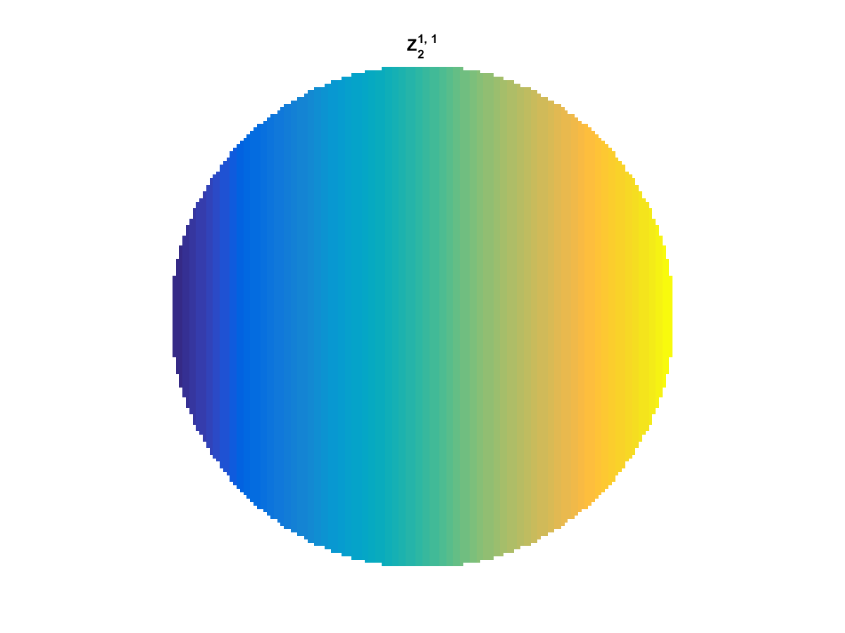
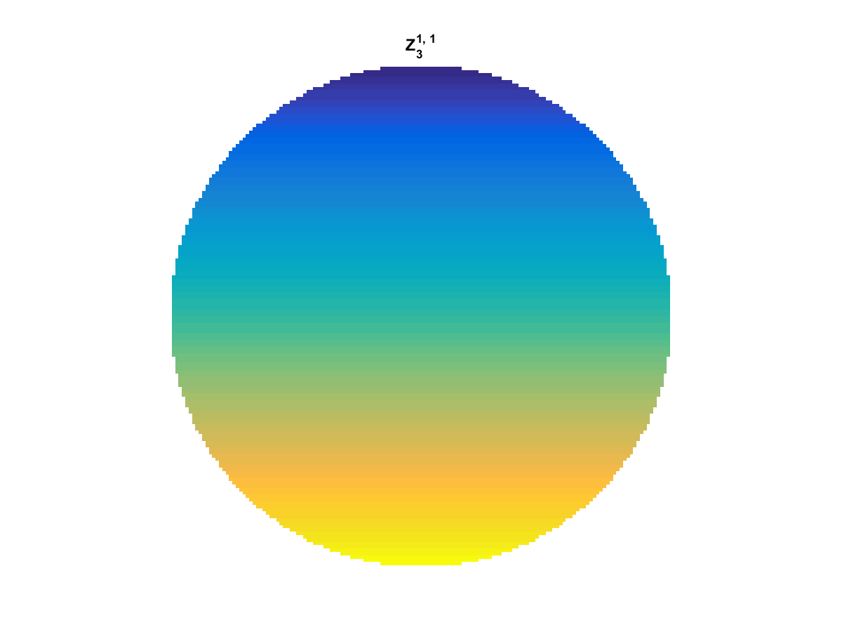
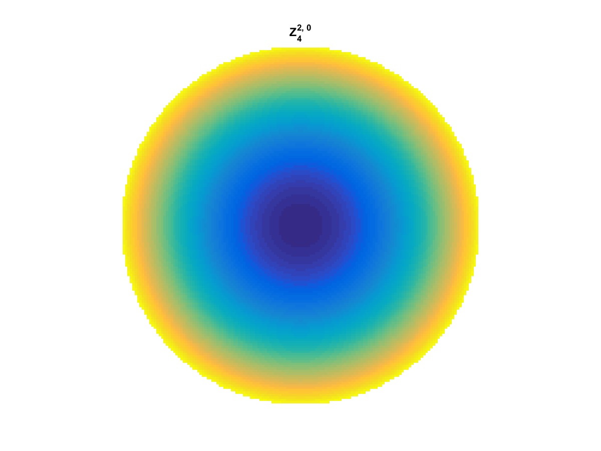
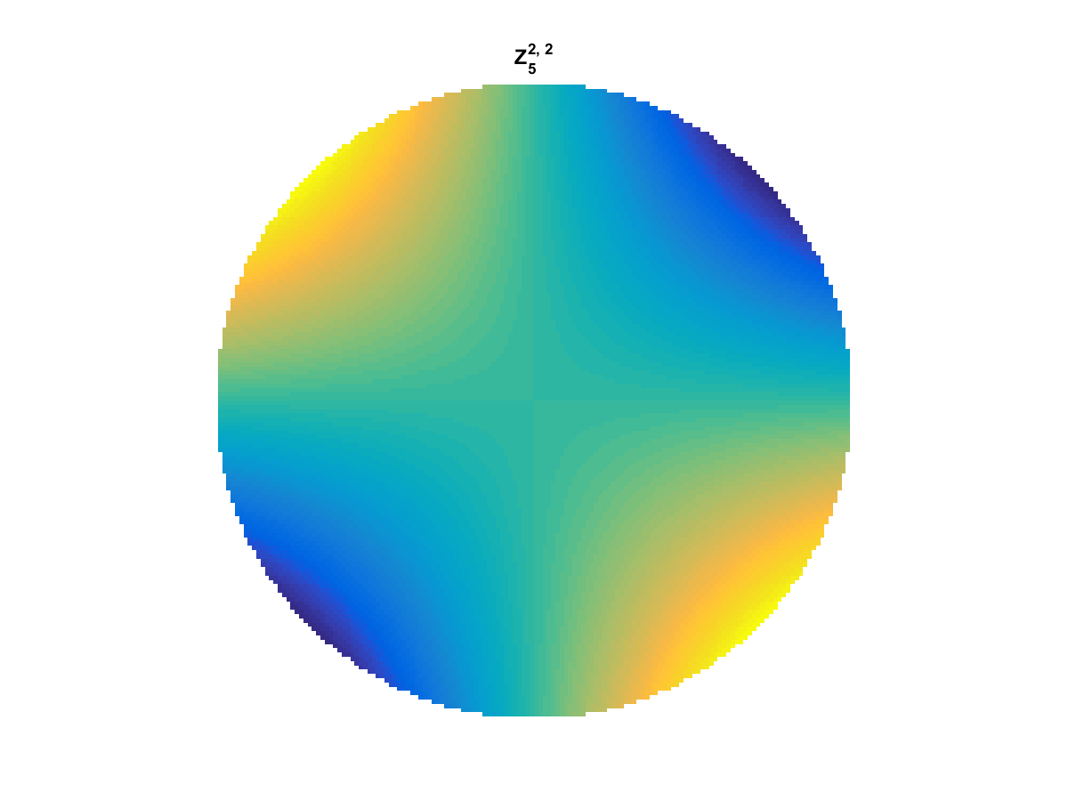
With Noll normalization. Certain polynomials have names. First is \(Z_1\), know as Piston as is often subtracted to study of single aperture systems. Next, \(Z_2\) and \(Z_3\) are ramps that are called tilt and cause displacement. \(Z_4\) is a centered ring structure known as defocus while \(Z_5\) and \(Z_6\) are astigmatism, \(Z_7\) and \(Z_8\) are coma, and \(Z_{11}\) is spherical aberration.
They can be imaged as follows:

All created using the following code:
function result = z_cart(i,m,n, x,y)
%Z_POL result the zernike polynomial specified in cartesian coordinates

% calculate the polar coords of each point and use z_pol:
r = (x.^2 + y.^2).^(1/2);
thta = atan2(y,x);

result = z_pol(i,m,n,r,thta);

end

function result = z_pol(i, m,n, r,t)
%Z_POL result the zernike polynomial specified in polar coordinates

if(m==0)
    result = radial_fun(0,n,r);
else
    if mod(i,2) == 0 % is even
        term2 = cos(m*t);
    else
        term2 = sin(m*t);
    end

    result = sqrt(n+1)*radial_fun(m,n,r).*term2;
end

end

function result = radial_fun(m,n,r)
%RADIAL_FUN calculate the radial function values for m,n, and r specified
result = 0;

for s = 0:(n-m)/2
    result = result + (-1)^s *factorial(n-s)/ ...
        (factorial(s)*factorial((n+m)/2 -s)*factorial((n-m)/2-s)) *...
        r.^(n-2*s);
end
end

Matlab has incorporated GPU processing on the parallel computing toolbox and you can create GPU array objects using the gpuArray(…) function in MATLAB. I created a brief script to compare matrix multiply of a 2048 x 2048 matrix against a vector. Ordinarily, the CPU operations see reasonable speedup (~2x) from moving from double to single precision values. However, moving to the GPU implementation results in a speedup of 6.8x for Double and 5.6x for Single! This means that if you can take a matrix-vector multiply that is double precision and convert it to single precision GPU version, you may see a gain of nearly 14x.
The following we generated in Matlab R2014b on an i7-4770 3.5 Ghz CPU (8 CPUs) with 16GB Ram and a Geforce GTX 750.
 The next step is to evaluate speed of the gpuArray on a basic L1 Optimization set—l1 magic.
The code used to generate this data is as follows:
allTypes = {'Double', 'gpuArrayDouble', 'Single', 'gpuArraySingle'};
allTimes = nan(length(allTypes),1);

n = 2048;       % size of operation for Ax
num_mc = 2^10;  % number monte carlo runs to compute time average of runs

randn('seed', 1982);
Am = randn(n,n);
xm = randn(n,1);

for ind_type = 1:length(allTypes)

    myType = allTypes{ind_type};

    switch lower(myType)
        case 'double'
            A = double(Am);
            x = double(xm);
        case 'single'
            A = single(Am);
            x = single(xm);
        case 'gpuarraydouble'
            A = gpuArray(Am);
            x = gpuArray(xm);
        case 'gpuarraysingle'
            A = gpuArray(single(Am));
            x = gpuArray(single(xm));
        otherwise
            error('Unknown type');
    end

    tic
    for ind_mc = 1:num_mc
        y = A*x;
    end
    allTimes(ind_type) =  toc/num_mc;

end

%% Display the results
figure(34);
clf;
bar(allTimes*1000);
set(gca, 'xticklabel', allTypes, 'color', [1 1 1]*.97);
title(['Timing of CPU and GPU in M' version('-release')]);
xlabel('Type');
ylabel('Time (ms)');
grid on

%%
figure(35);
clf;
speedupLabels = {('Double to Single') , ...
                 ('Double to gpuDouble'), ...
                 ('Single to gpuSingle'), ...
                 'Double to gpuSingle'};
bar([allTimes(1)/allTimes(3), allTimes(1)/allTimes(2),  ...
    allTimes(3)/allTimes(4), allTimes(1)/allTimes(4)]);
set(gca, 'xticklabelrotation', 15, 'xticklabel', speedupLabels, 'color', [1 1 1]*.97);
title(['Speedup of CPU and GPU in M' version('-release')]);
xlabel('Type');
ylabel('Speedup');
grid on