Introductory Plots for Deconvolution

A basic test was run to begin to gain some intuition on the affects of a spatially varying convolution kernels. The goal is to divide the image into sections, apply a different kernel on the different sections, then deconvolve using the correct and/or incorrect kernel. I used Lucy-Richardson deconvolution as well as blind deconvolution.

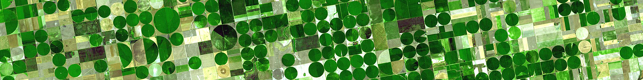
The Creative Commons Kansas Crops image was taken from Wikipedia because it 1) is similar to an image of interest, 2) varied in texture while having some quality sharpness, 3) maintained similar features throughout.

OriginalImage
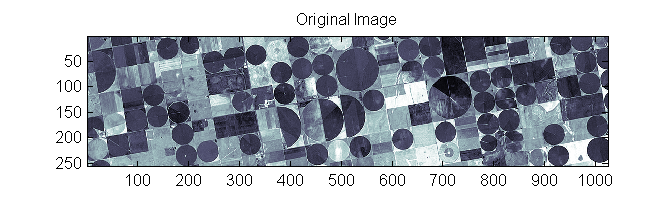
Box Kernels 1 through 4 were created of size [2, 10, 18, 26] (that’s 2+8*(ind-1)) in order to create a set of blurred images as follows:BlurImages1to4Lucy-Richardson deconvolution was then used to deconvolve the blurred image back into the original by providing it the true kernel used for each image and 100 iterations. While the larger kernels are more challenging, the images to quite well at 100 iterations:

DeconvolveLucyProperIter100But what happens when the wrong kernel is used? The answer is: very bad things. Here is an example of the output of running Lucy-Richarddon on the Original Image blurred with kernel 2 but telling Lucy-R to deconvolve using kernel 4:

Image2LucyKernel4
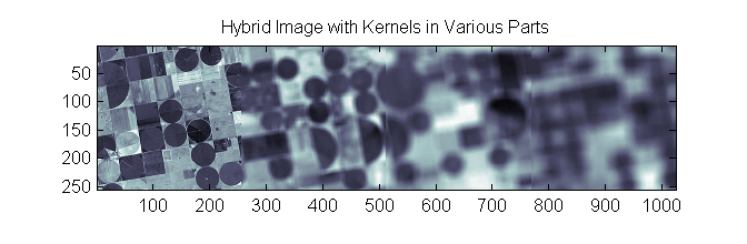
To further explore, I created a hybrid image that took 256 x 256 blocks from independent regions of the individual blurred images 1-4 and concatenated them to create a single image with difference independent blurs:

TheHybridImageThe Lucy-Richardson Deconv. routine was then run and given each of the for 4 kernels:

HybridWithVariousKernelsRunAgainstItLucyIter100The results are consistent with the individual Image2/Kernel4 combo shown above with the added problem that the transition between the two regions is quite abrupt.

A final test was run showing the results of blind deconvolution on the hybrid image starting with Kernel1 through kernel4 as an initial guess. The results are similar:

HybridWithVariousStartingKernelsAndBlindIter100

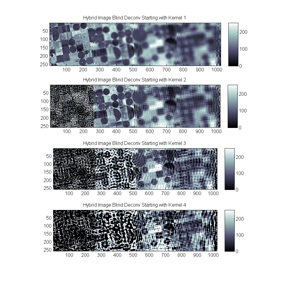
As noted, a certain unkindness has been done to the deconvolution in both the Lucy and the Blind case. Since the hybrid was created with abrupt changes from one kernel to the next we introduce a visible discontinuity on the border of the regions. While the transition will always be there this results in significant problems in the frequency domain and causes ringing in spatial domain as well.

Further improvements will be to begin to address the non-homogeneity of the blurring kernel directly as well as consider the transition regions.

Cholesky MKL Baseline

This article will attempt to establish a performance baseline for creating a custom Cholesky decomposition in MATLAB through the use of MEX and the Intel Math Kernel Library (MKL). In the past I showed a basic and block Cholesky decomposition to find the upper triangular decomposition of a Hermitian matrix A such that A = L’L. The block performed substantially better than a single term operation but still  not as good as MATLAB R2013a Intrinsic Chol(…) function. The times worked out to be that the non-blocking Cholesky decomposition in MATLAB was about 200x slower than MATLAB and the Blocking was about 7x slower. Further work by Chris Turnes in porting his code to C++ showed substantial gains, and using BLAS routines rather than naive C++ improved things further. However, parity with MATLAB was still not achieved. Sources indicate that MATLAB uses the MKL internally, so I correctly expected that calling the MKL LAPACK Chol(…)-equivalent function should yield equivalent results. However, the operation is blazing fast and so care must be taken with memory management and copies in order to reach parity with MATLAB.

The Intel MKL is a fast mathematics library from Intel that includes full implementations of BLAS, LAPACK, FFT, and other operations. It widely utilizes clever optimizations and Single Instruction Multiple Data (SIMD) operations like SSE. The LAPACK routine we are interested in is

int dpotrf(char *uplo, int *n, double *a, int*lda, int *info);

where dpotrf(…) is the double precision (“d”), symmetric or Hermitian positive definitite (“po”) triangular factorization (“trf”) LAPACK routine. We wish to create an upper triangular factorization by setting uplo to “U” for upper, the dimension n and lda to the size of the matrix, and the data pointer a to a COPY of the matrix to factor because this factorization is going to happen in place.

It turns out the copy operation is best done but copying only the upper triangular part of the matrix A. A naive copy using

plhs[0] = mxDuplicateArray(A);

is a poor choice for two reasons. First, the function dpotrf(…) writes its results only in the upper triangular portion of result and leaves the rest of the matrix as is. The result is that you must zero out the lower triangular part in C++ or call triu(C) on the resulting triangular factorization in MATLAB. Doing a FULL copy and then calling triu(…) results in code that is about 15% slower than only copying the parts of A you need and then dropping triu(…). The proper code for extracting the upper part of a given matrix was written by Turnes as:

plhs[0] = mxCreateDoubleMatrix(n, n, mxREAL);
double *data = mxGetPr(plhs[0]), *prIn = mxGetPr(prhs[0]);
for (int i = 0; i < n; i++)
    memcpy(data + i*n, prIn + i*n, sizeof(double)*(i+1));

Once this is done, the LAPACK routine can be executed. As it turns out, you can run either a full copy of MKL or plug into the MATLAB version by compiling with mex and the -lmwlapack option like so:

mex cholchol.cpp -lmwlapack

Both reach parity with MATLAB for large sizes. This means that we may be able to reach parity with MATLAB using MEX code provided that we use optimized BLAS routines. For example, at size 2048 x 2048 real matrix, I obtain the following timing:

  1. Time cholchol(…) MEX/MKL:  0.1315 s
  2. Time MATLAB: 0.1302 s

Next, I may consider implementing the block Cholesky decomposition in C++ using basic BLAS and the rank-k updates from MKL in order to attempt to achieve parity with more custom code.

You can download the main cholchol(…) code here.

And a comparison of times for various sizes:

CholeskyMKLComparison

This code as run on Sonata:

  1. Motherboard: Gigabyte X58U-UD3R
  2. Processor: Intel Core i7 950 @ 3.07 Ghz (8CPU)
  3. Memory: 8GB
  4. OS: Windows 7
  5. MATLAB: R2013A
  6. Compiler: Visual Studio 2012
  7. MKL: Intel Composer XE 2013 SP1

Block Cholesky Decomposition

A substantial improvement on the prior Cholesky decomposition can be made by using blocks rather than recursing on the scalar. This allows us to work in much large chunks and even makes the recursive formulation competitive.

Here is the recursive code:


function U = chol_sec_block(A)
% Author: Stephen Conover
% Date: January 2014
% This function uses a block formulation to recursively computer the
% cholesky decomposition of a NxN hermitian matrix A.

blockSize  = min(96, length(A));

if(isempty(A))
U = [];
return;
end;

U = zeros(size(A));

% Computer the blocks:
Utl = chol_sec_nr(A(1:blockSize, 1:blockSize));
Utr = (Utl^-1)'*A(1:blockSize, blockSize+1:end);

U(1:blockSize,1:blockSize) = Utl;
U(1:blockSize,blockSize+1:end) = Utr;

% Do the recursion.
Sbr = A(blockSize+1:end, blockSize+1:end) - Utr'*Utr;
U(blockSize+1:end, blockSize+1:end) = chol_sec_block(Sbr);

end

and here is the non-recursive:

function U = chol_sec_nr_block(A)
% Author: Stephen Conover
% Date: January 2014
% This function uses a block formulation to non-recursively computer the
% cholesky decomposition of a NxN hermitian matrix A.

% check for Empty:
if(isempty(A))
U = [];
return;
end;

% Intialize output:
N = length(A);
U = zeros(size(A));

blockSize = 96;
myOffset = -blockSize;
inds = 1:blockSize;

% Loop through each chunk of blocksize:
for n = 1:N/blockSize

myOffset = (n-1)*blockSize;

Utl = chol_sec_nr(A(myOffset + inds, myOffset + inds));
Utr = (Utl^-1)'*A(myOffset + inds, (n*blockSize+1):N);

U(inds + myOffset,inds+myOffset) = Utl;
U(myOffset + inds, (n*blockSize+1):N) = Utr;

Sbr = A(myOffset+1+blockSize:N, myOffset+1+blockSize:N) - Utr'*Utr;
A(myOffset+1+blockSize:N, myOffset+1+blockSize:N)  = Sbr;

end

% finish off the rest of the computation < blockSize int he bottom right:
if(mod(N, blockSize) > 0)
U(myOffset+1+blockSize:end, myOffset+1+blockSize:end) = chol_sec_nr(A(myOffset+1+blockSize:end, myOffset+1+blockSize:end));
end

end

The following plot compares the original scalar formulation, the new block recursive/non-recursive formulation, and the MATLAB intrinsic. The MATLAB intrinsic still spanks the scripting code but I believe we may see this come close to parity when it is implemented in C++.

Cholesky Speed ComparisonsExample speeds at 1500 x 1500 are:

  1. Original Custom Recursive Scalar Decomposition time: 15.79s
  2. Custom Recursive Cholesky Block Decomposition time: 0.3571s
  3. Custom Non-Recursive Cholesky Block Decomposition time: 0.3384s
  4. MATLAB Intrinsic Cholesky Decomposition time: 0.0510s

Cholesky Decomposition

The Cholesky decomposition takes a Hermitian, positive definite matrix and expresses it as UU’—a highly efficient decomposition for solving system of equations.

We want to decompose the Hermitian positive definite \(A\) into an upper triangular matrix \(U\) such that \(A=U^HU\). Then we can write
\[A=U^HU = \begin{pmatrix} \alpha_{11} & a_{12} \\ a_{12}^H & A_{2,2} \end{pmatrix} = \begin{pmatrix} \bar{\upsilon}_{11} & 0 \\ u_{12}^H & U_{22}^H \end{pmatrix} \begin{pmatrix} \upsilon_{11} & u_{12} \\ 0 & U_{22} \end{pmatrix}\]
and thus
\[ A = \begin{pmatrix} \left| \upsilon_{11} \right| ^2 & \bar{\upsilon}_{11}u_{12} \\ \upsilon_{11} u_{12}^H & u_{12}^H u_{12} + U_{22}^H U_{22} \end{pmatrix} \]
we can solve for the components to get
\[\upsilon_{11} = \sqrt{\alpha_{11}}\]\[u_{12} = a_{12} / \upsilon_{11} \]\[S_{22} = A_{22} – u_{12}^Hu_{12}\]
where \(S_{22}\) is the Schur Complement.

The function chol(…) in MATLAB will create the Cholesky decomposition but their implementation is hidden. A custom implementation is as follows:


function U = chol_sec(A)

    if(isempty(A))
        U = [];
        return;
    end;

    U = zeros(size(A));

    u11 = A(1,1)^(1/2);
    u12 = A(1,2:end)/u11;

    U(1,1) = u11;
    U(1,2:end) = u12;

    S22 = A(2:end, 2:end) - u12'*u12;
    U(2:end, 2:end) = chol_sec(S22);

end

This code can be exercised using the following:

% Make a test matrix:
randn('seed', 1982);
A = randn(6);% + randn(6)*i;
A= A'*A; % Make it symmetric

% Do the thing:
disp('My Result:');
U = chol_sec(A)

% And run the matlab intrinsic to be sure we got the right result:
disp('MATLAB''s Result');
U_matlab = chol(A)

err = norm(U - U_matlab)

Also, a MATLAB tends to die with large dimensions because the recursion depth is limited. To avoid this you can use a non-recursive formulation as follows:

function U = chol_nr_sec(A)

U = zeros(size(A));

for n = 1:length(A)
    
    u11 = A(n,n)^(1/2);
    u12 = A(n,(1+n):end)/u11;
    
    U(n,n) = u11;
    U(n,(1+n):end) = u12;
    
    A((n+1):end, (n+1):end) = A((n+1):end, (n+1):end) - u12'*u12;
end

end

The non-recursive formulation is about 33% faster than the recursive formulation on my system with MATLAB 2013a, but is about 200 times slower than the intrinsic formulation.

  1. Custom Recursive Cholesky Decomposition time: 0.3063s
  2. Custom Non-Recursive Cholesky Decomposition time: 0.1908s
  3. MATLAB Intrinsic Cholesky Decomposition time: 0.0020s