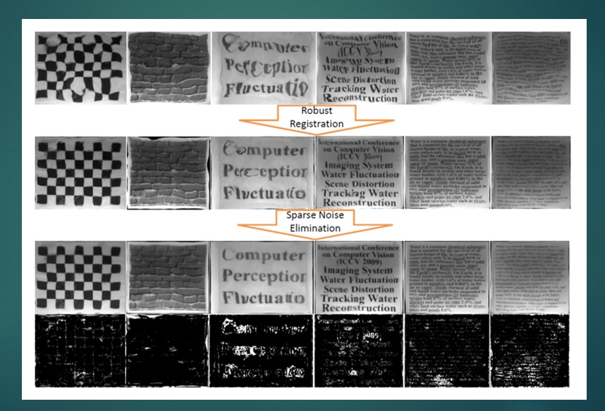
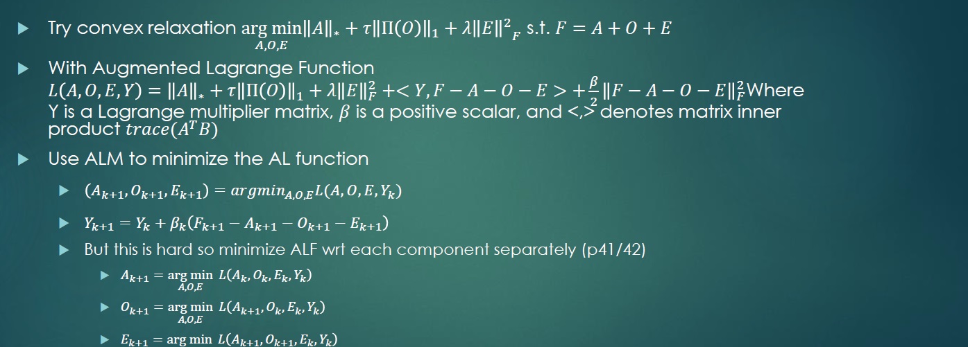
Presentation on Turbulence Mitigation using low rank estimation.
Download: Robust Subspace Estimation Using Low-Rank Optimization
 .
.
Development, Research, Other Stuff
Presentation on Turbulence Mitigation using low rank estimation.
Download: Robust Subspace Estimation Using Low-Rank Optimization
.
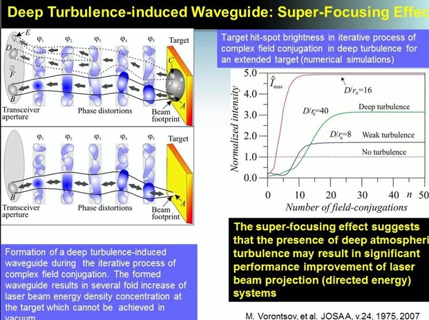
“Dr. Mikhail Vorontsov, Ph. D from the University of Dayton Electro-Optics Program presents a lecture titled “How Atmospheric Turbulence can be used to improve Optical Systems Performance” at the 2012 Spotlight on Technology, Arts, Research and Scholarship at the University of Dayton.”
Thanks to Clayton for sending this to me.
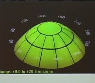
This is a great video from PhotoTechEDU GoogleTech talks by Eric Gross discussing the measurement and correction of optical aberrations through laser surgery. It discusses
Abnormalities in the eye can create similar wavefront aberrations as optical turbulence.
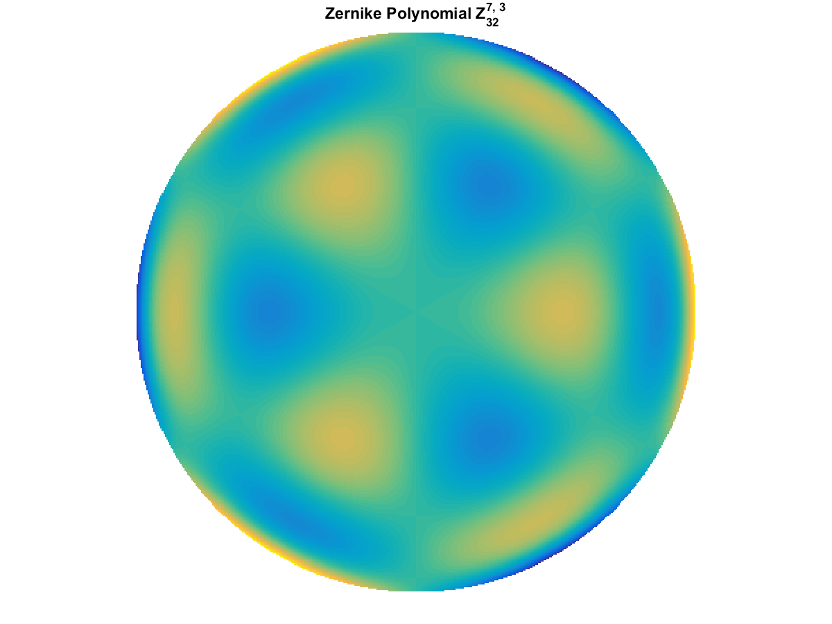
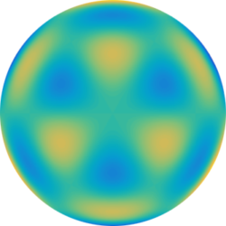
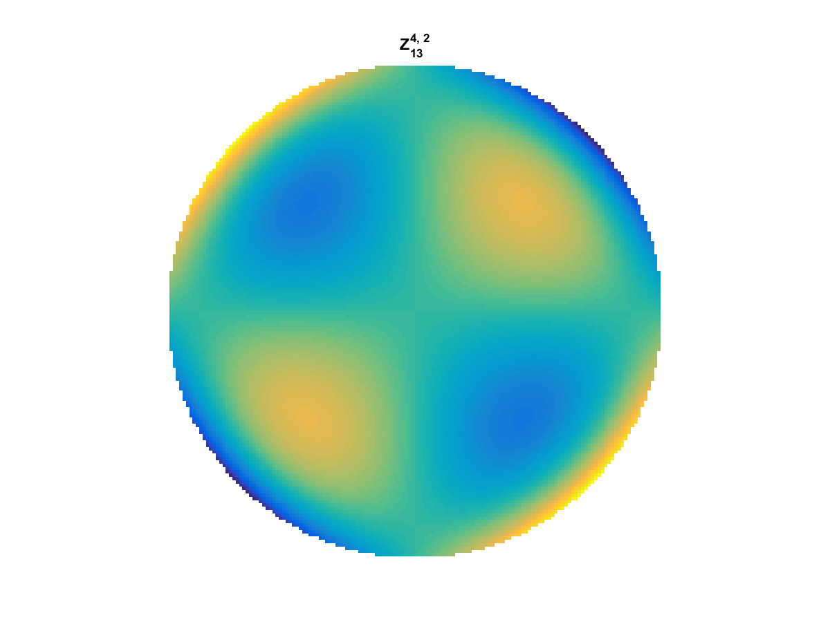
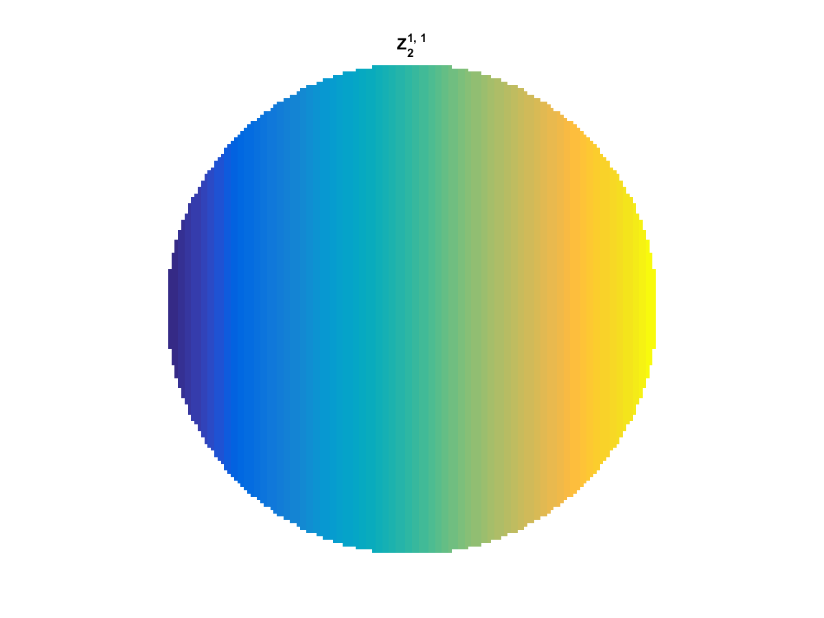
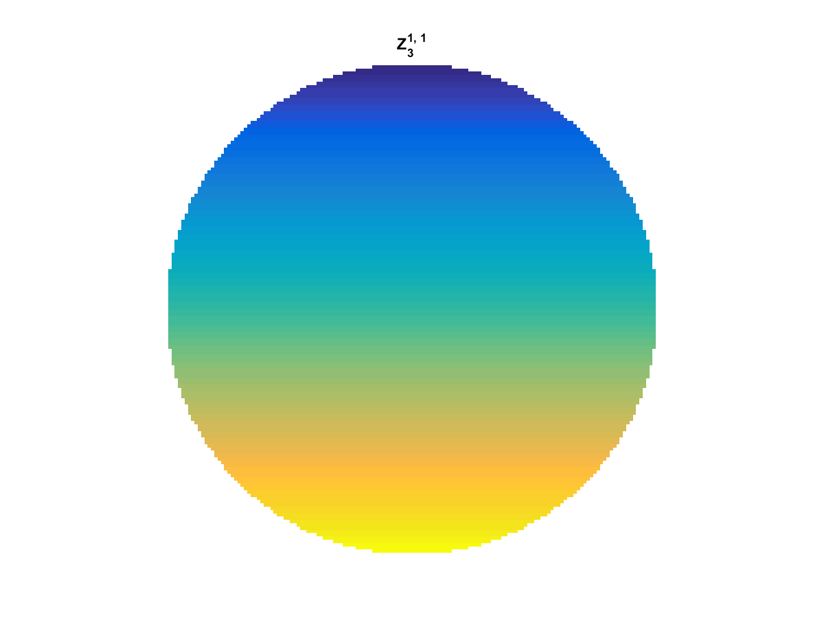
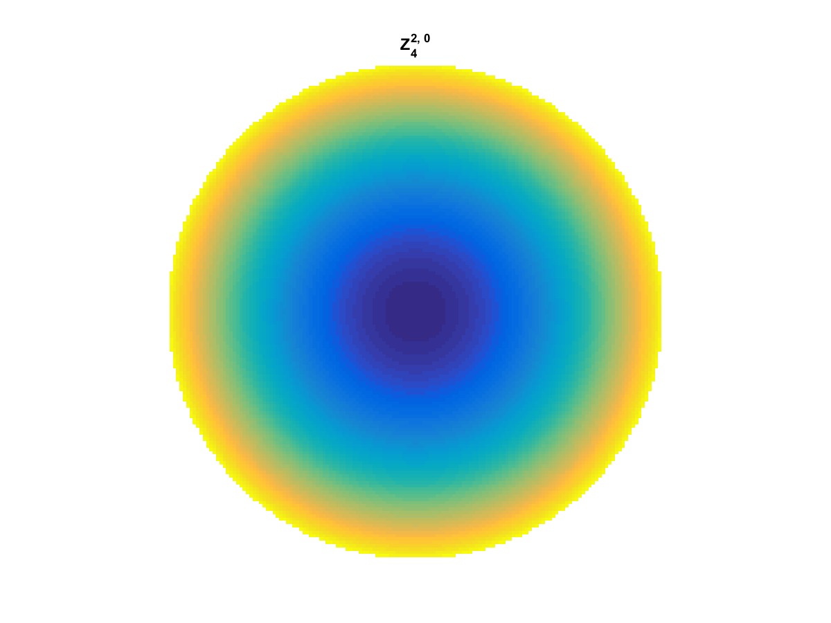
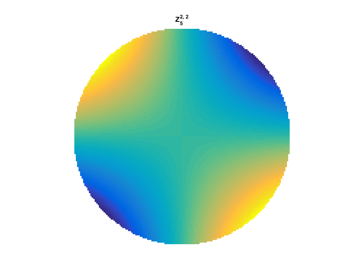
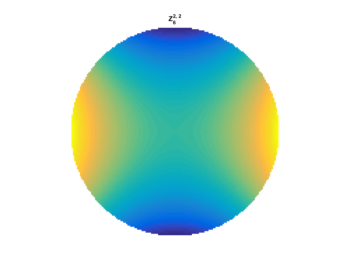
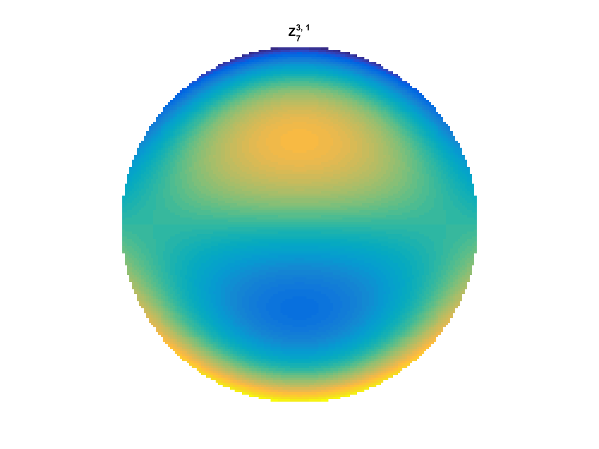
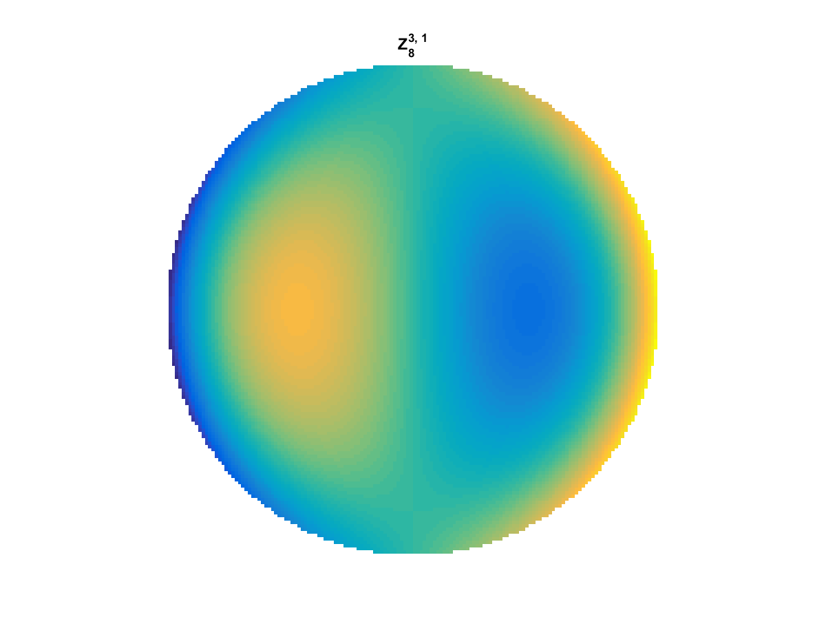
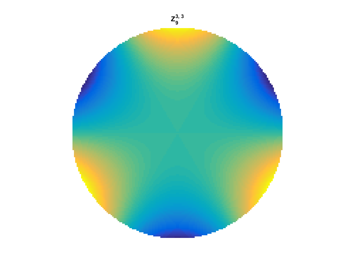
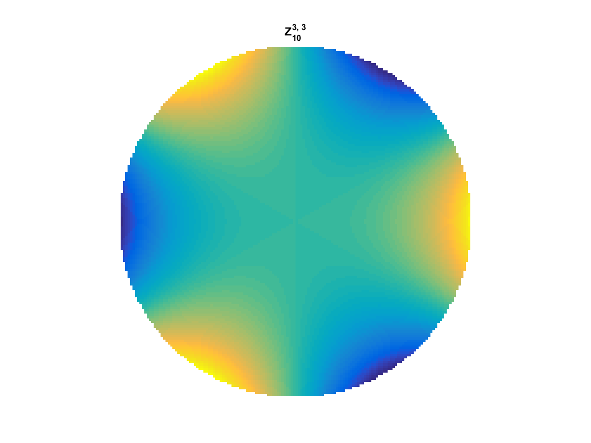
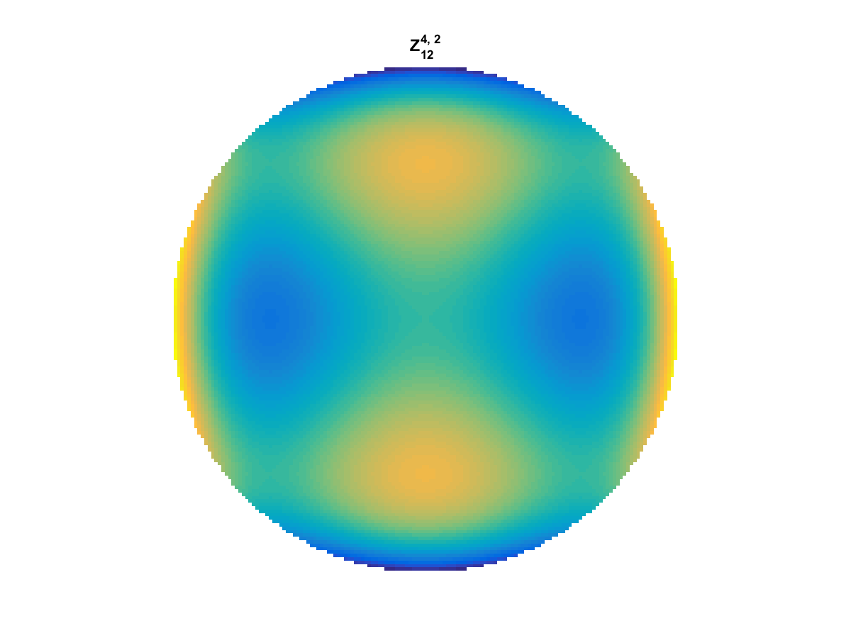
A quick implementation of of Zernike polynomials for modeling wavefront aberrations to to optical turbulence. Equations pulled from Michael Roggemann’s Imaging Through Turbulence.
Zernike polynomials are often used to model wavefront aberrations for various optics problems. The equations are expressed in polar coordinates, so to calculate the image we first convert a grid into polar coordinates using the relation
\(y = r\times sin(\theta) \)
\(r = \sqrt{x^2 + y^2} \)
\(\theta = tan^{-1}\frac{y}{x}\)
And then calculate the Zernike Polynomials as
\(Z_{i,even}(r,\theta) = \sqrt{n+1}R^m_n(r)cos(m\theta) \)
\(Z_{i,odd}(r,\theta) = \sqrt{n+1}R^m_n(r)sin(m\theta) \)
and \(Z_{i}(r,\theta) =R^0_n(r)\) if \(m=0\)
Where the functions \(R^m_n(r)\) are called Radial Functions are are calculated as
\(R^m_n(r) =\sum_{s=0}^{(n-m)/2} \frac{(-1)^s(n-s)!}{s![(n+m)/2 – s]![(n-m)/2 – s]!} r^{n-2s} \)
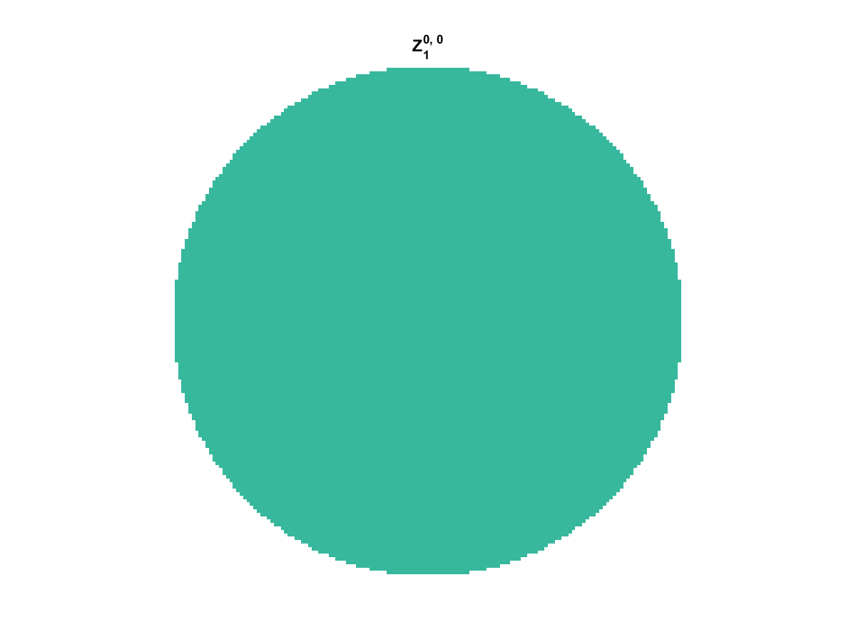
With Noll normalization. Certain polynomials have names. First is \(Z_1\), know as Piston as is often subtracted to study of single aperture systems. Next, \(Z_2\) and \(Z_3\) are ramps that are called tilt and cause displacement. \(Z_4\) is a centered ring structure known as defocus while \(Z_5\) and \(Z_6\) are astigmatism, \(Z_7\) and \(Z_8\) are coma, and \(Z_{11}\) is spherical aberration.
They can be imaged as follows:

All created using the following code:
function result = z_cart(i,m,n, x,y)
%Z_POL result the zernike polynomial specified in cartesian coordinates

% calculate the polar coords of each point and use z_pol:
r = (x.^2 + y.^2).^(1/2);
thta = atan2(y,x);

result = z_pol(i,m,n,r,thta);

end

function result = z_pol(i, m,n, r,t)
%Z_POL result the zernike polynomial specified in polar coordinates

if(m==0)
    result = radial_fun(0,n,r);
else
    if mod(i,2) == 0 % is even
        term2 = cos(m*t);
    else
        term2 = sin(m*t);
    end

    result = sqrt(n+1)*radial_fun(m,n,r).*term2;
end

end

function result = radial_fun(m,n,r)
%RADIAL_FUN calculate the radial function values for m,n, and r specified
result = 0;

for s = 0:(n-m)/2
    result = result + (-1)^s *factorial(n-s)/ ...
        (factorial(s)*factorial((n+m)/2 -s)*factorial((n-m)/2-s)) *...
        r.^(n-2*s);
end
end